Tuning PID Controllers with Automatic Differentiation

PID controllers are the workhorses of industrial control. They are simple enough to fit on a microcontroller, yet surprisingly effective across a wide range of systems. The catch is that tuning them well takes time and, if you are being honest, a fair amount of intuition. Classic recipes like Ziegler-Nichols are fast but often leave performance on the table. Model-free autotuning approaches work but can require live experiments on the real plant.

Here is a different take: write down a differentiable simulation of your system, define a loss that captures what “good control” means to you, and let gradient descent find the gains. Automatic differentiation handles the calculus; you just specify the objective.

This post walks through exactly that, using JAX¹. The controller structure follows the practical implementation guidelines of Sundström et al.²

The Example: A Second-Order Mass-Spring-Damper

The plant is a linear mass-spring-damper:

m\ddot{x} + c\dot{x} + kx = u(t)

with mass $m = 1\,\text{kg}$ , damping $c = 0.5\,\text{N·s/m}$ , and spring stiffness $k = 2\,\text{N/m}$ . The PID controller drives the position $x$ to a unit step setpoint.

This system has a natural frequency of $\omega_n = \sqrt{k/m} \approx 1.41\,\text{rad/s}$ and a damping ratio of $\zeta = c/(2\sqrt{mk}) \approx 0.18$ , so the open-loop step response is lightly damped and oscillatory — a good stress test for the tuning method.

The Incremental (Velocity) Form

Rather than computing the control output $u$ directly at each step, the simulation uses the incremental (or velocity) form: only the increment $\Delta u$ is computed, and the output is accumulated as $u[k] = u[k-1] + \Delta u[k]$ .

This structure has several practical advantages over the position form. Actuator saturation and bumpless switching are easier to handle because the accumulator naturally keeps track of where the integrator state is. There is also no integral wind-up from the proportional or derivative paths — only the explicit integral increment $\Delta u_i$ can cause wind-up.

Setpoint weighting

A standard PID controller applies the setpoint equally to all three terms. In practice it is often better to split this: let the proportional and derivative paths see a weighted version of the setpoint, while the integral path always sees the full error.

Two weights $b$ and $c$ parameterise this:

e_p[k] = b\,r - y[k], \qquad e_d[k] = c\,r - y[k], \qquad e[k] = r - y[k]

Setting $b < 1$ reduces the proportional kick when the setpoint steps, giving a smoother response without sacrificing integral action. Setting $c = 0$ makes the derivative act only on measurement changes — eliminating the large derivative spike that would otherwise appear at $t = 0$ when $r$ jumps discontinuously.

Derivative approximation

Rather than differentiating the error, the derivative is approximated separately for $r$ and $y$ via finite differences:

\dot{r}[k] = \frac{r[k] - r[k-1]}{\Delta t}, \qquad \dot{y}[k] = \frac{y[k] - y[k-1]}{\Delta t}

The second-difference increments $\Delta\dot{r}[k] = \dot{r}[k] - \dot{r}[k-1]$ and $\Delta\dot{y}[k] = \dot{y}[k] - \dot{y}[k-1]$ then enter the derivative increment directly.

Discrete update equations

The full incremental update at step $k$ is:

\begin{aligned} \Delta u_p[k] &= K_p\bigl(b\,\Delta r[k] - \Delta y[k]\bigr) \\ \Delta u_i[k] &= K_i\,\Delta t\,e[k] \\ \Delta u_d[k] &= K_d\bigl(c\,\Delta\dot{r}[k] - \Delta\dot{y}[k]\bigr) \\ u_{\text{raw}}[k] &= u[k-1] + \Delta u_p[k] + \Delta u_i[k] + \Delta u_d[k] \end{aligned}

where $\Delta r[k] = r[k] - r[k-1]$ and $\Delta y[k] = y[k] - y[k-1]$ .

For a constant setpoint $\Delta r = 0$ on every step after the initial one, so the proportional increment reduces to $-K_p\,\Delta y$ and only responds to how the output is changing. The integral term $K_i\,\Delta t\,e[k]$ carries the absolute error information needed to eliminate steady-state offset.

The plant is integrated with semi-implicit Euler (velocity updated before position), which is slightly more stable than explicit Euler for oscillatory systems at the same step size $\Delta t = 0.01\,\text{s}$ .

Saturation and Anti-Windup

Rate-limited bounds

Rather than applying fixed saturation limits $[u_{\min},\, u_{\max}]$ directly, the active bounds at each step are tightened by a rate constraint on the previous output $u_s[k-1]$ :

\hat{u}_{\min}[k] = \max\!\bigl(u_{\min},\; u_s[k-1] + \Delta t\,\dot{u}_{\min}\bigr), \quad \hat{u}_{\max}[k] = \min\!\bigl(u_{\max},\; u_s[k-1] + \Delta t\,\dot{u}_{\max}\bigr)

This limits how fast the actuator output can change between steps, independently of the absolute limits. In the current simulation the rate limits are set large enough to be inactive, but the structure is in place for the general case.

Anti-windup by soft pull-back

After computing $u_{\text{raw}}$ , a soft correction pulls the signal back toward the feasible region before the hard clip:

u_s = \text{clip}(u_{\text{raw}},\; \hat{u}_{\min},\; \hat{u}_{\max})

u \leftarrow u_{\text{raw}} - \frac{\Delta t}{T_t}\bigl(u_{\text{raw}} - u_s\bigr)

u[k] = \text{clip}(u,\; \hat{u}_{\min},\; \hat{u}_{\max})

When the signal is within bounds $u_s = u_{\text{raw}}$ and the correction vanishes. When saturated, the correction partially unwinds the accumulator at a rate governed by the time constant $T_t$ . The state carried forward is $u$ (after soft correction, before the final hard clip), so the integrator is reset smoothly rather than hard-clamped. The hard clip on $u[k]$ ensures the plant never sees an out-of-range command.

The Loss Function

The objective combines four terms:

\mathcal{L} = \underbrace{\sum_{n=0}^{N} w_n\, e_n^2\,\Delta t}_{\text{weighted tracking}} + \underbrace{10 \cdot \frac{1}{N}\sum_n \max(|e_n| - 0.01,\, 0)}_{\text{tail penalty}} + \underbrace{10^{-2}\!\sum_n u_n^2\,\Delta t}_{\text{effort}} + \underbrace{10^{-2} \cdot \frac{1}{N}\sum_n\left|\sum_{j\le n} e_j\,\Delta t\right|}_{\text{integral penalty}}

where $w_n = 1 + 5\,(t_n / T)^2$ and $T = 10\,\text{s}$ .

Weighted tracking is the dominant term. The quadratic time-weighting $w_n$ goes from $1$ at $t = 0$ to $6$ at $t = T$ , so errors near the end of the simulation are penalised six times more than early-transient errors.

Tail penalty adds a hard push toward zero once the error exceeds $0.01\,\text{m}$ . It acts as a deadband: below the threshold the gradient from this term vanishes, preventing the optimiser from over-tightening in the noise-free simulation.

Effort penalises large control signals with a small coefficient ( $10^{-2}$ ), discouraging unnecessarily aggressive gains.

Integral penalty discourages large integral accumulation, which indirectly limits integral wind-up.

Why JAX?

JAX’s jit + grad pipeline means the gradient computation costs roughly the same as two forward passes — that is the magic of reverse-mode AD. With jax.lax.scan you can unroll the simulation loop without materialising every intermediate in Python, keeping compilation time and memory under control even for long horizons.

There are no finite-difference approximations and no symbolic manipulations. The gradients are numerically exact (up to floating point) regardless of the complexity of the integrator or the loss. Crucially, jnp.clip is differentiable in JAX: its subgradient is zero in the saturated region and one elsewhere, so the optimizer receives a correct signal even when the saturation bounds are active.

Optimisation Setup

The optimised parameters are $[K_p,\, K_i,\, K_d]$ , initialised at $[1, 0, 0]$ . The setpoint weights $b = 1$ and $c = 0.5$ are treated as fixed constants — the gradient is taken only with respect to the three gains. This decoupling is intentional: $b$ and $c$ encode a design choice about how aggressively the controller should react to setpoint steps, and are better set by the engineer than discovered by gradient descent.

Adam runs for 3000 iterations with a cosine-decaying learning rate starting at $0.1$ . The decay is important: without it the gains could grow indefinitely, since larger gains always reduce the time-weighted tracking error. The cosine schedule lets the optimiser move fast early and then freeze the gains as the learning rate approaches zero.

Results

Step Response Comparison

Step response comparison

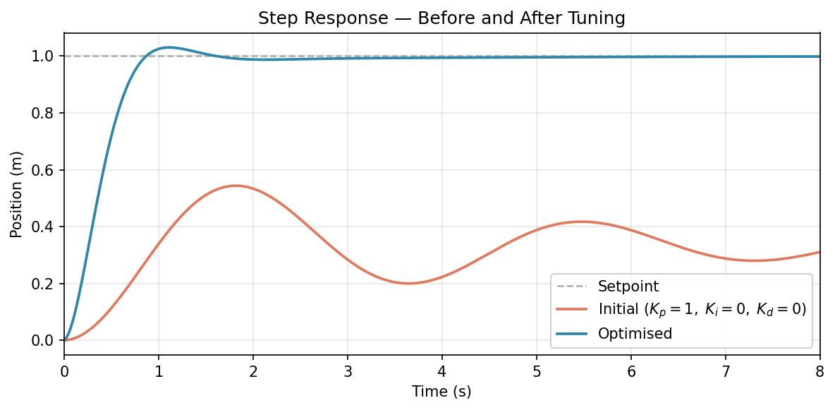
Orange is the initial controller ( $K_p = 1,\, K_i = 0,\, K_d = 0$ ). With the incremental form and no integral action, the controller accumulates a small control output on the first step (proportional kick from the setpoint step) and then only reacts to changes in the output — there is no mechanism to correct the residual position error once the output stops moving, so the response plateaus well below the setpoint.

Blue is the optimised controller. Integral action is the key difference: the $K_i\,\Delta t\,e[k]$ term keeps injecting a correction proportional to the current error, driving the output to the setpoint and holding it there.

Loss Curve

The loss drops by almost three orders of magnitude over 3000 iterations.

Loss over iterations

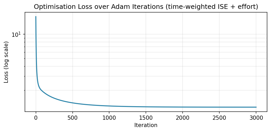
The steepest descent happens in the first few hundred iterations when the learning rate is near its peak value. After roughly iteration 1000 the cosine schedule has reduced the learning rate significantly and the curve flattens, indicating convergence.

Gain Trajectories

PID gain trajectories

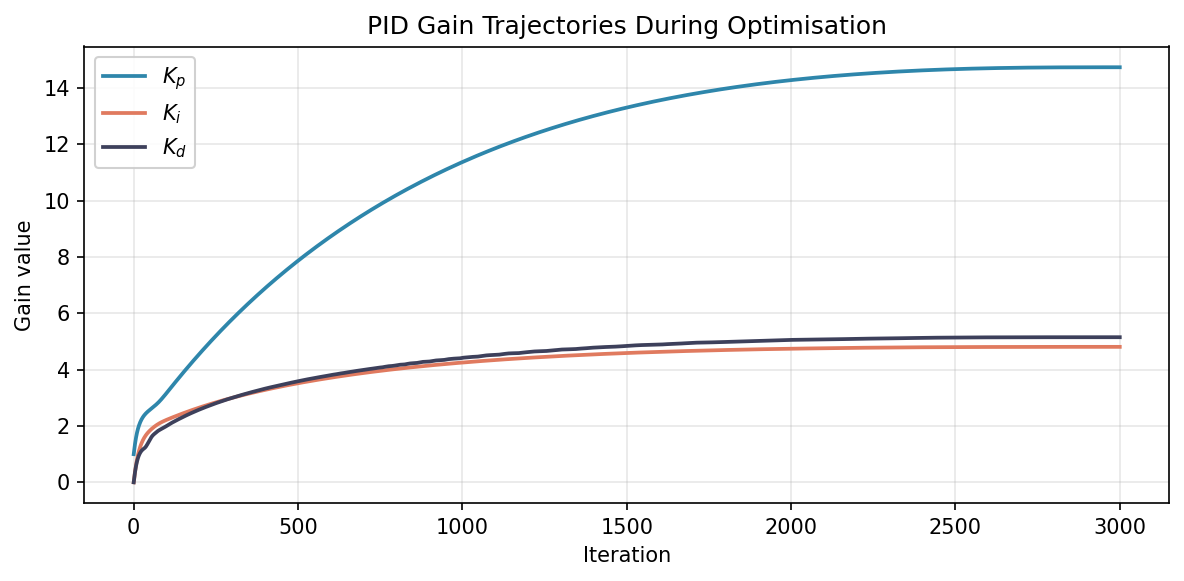
$K_p$ and $K_d$ respond immediately — they act on the current output change and its rate, so their gradient signal is strong and direct from the first step. $K_i$ lags because its effect accumulates over the entire trajectory; the gradient signal reaching it is more diffuse and takes longer to build up.

All three curves flatten as the cosine schedule drives the learning rate toward zero — a clean visual signature of convergence rather than a hard stop.

Tracking Error

Tracking error

Orange (initial, $K_i = 0$ ): the error settles to a non-zero constant. In the incremental form, once the plant reaches a pseudo-equilibrium the output increments vanish ( $\Delta y \approx 0$ ) and the control signal stops changing — locking in whatever offset remains.

Blue (optimised): the error oscillates briefly during the transient then decays to zero. The integral action is the mechanism: as long as $e[k] \neq 0$ , $\Delta u_i = K_i\,\Delta t\,e[k]$ keeps nudging the control output, and the accumulator only stops changing when the error is truly zero.

Control Effort

Control effort

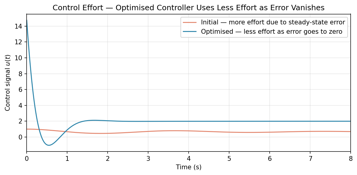
At $t = 0$ the controller sees a step in $r$ from $0$ to $1$ : $\Delta r = 1$ , $\Delta y = 0$ , so $\Delta u_p = K_p \cdot b \cdot 1$ . This is a finite proportional kick scaled by the setpoint weight $b$ . There is no derivative spike: since $c = 0.5$ and $\Delta\dot{r} = 0$ after the first step, the derivative increment is $-K_d\,\Delta\dot{y}$ — acting only on how the measurement is accelerating, not on the setpoint jump.

After the transient the optimised control signal settles to approximately $2\,\text{N}$ , which is the spring force $k \cdot x_{ss} = 2 \cdot 1\,\text{N}$ needed to hold the mass at $x = 1\,\text{m}$ .

Practical Considerations

Setpoint weights as design parameters. $b$ and $c$ control the trade-off between setpoint tracking aggressiveness and smooth transients. $b < 1$ softens the proportional response to reference steps. $c = 0$ turns the derivative into pure derivative-on-measurement, removing any setpoint-related derivative kick entirely. These are typically tuned by the engineer rather than optimised, because gradient descent can satisfy them in unintended ways (e.g. by exploiting the interaction between $b$ and $K_p$ ).

Anti-windup time constant. $T_t$ governs how quickly the integrator is unwound when the actuator saturates. A small $T_t$ (aggressive reset) can introduce instability if the plant is slow to respond. A value in the range $\sqrt{K_p/K_i}$ to the closed-loop settling time is a common practical starting point. Here $T_t = T_{\text{end}} = 10\,\text{s}$ as a loose default.

Simulation fidelity. Gradient-based tuning is only as good as your model. If the simulation drifts significantly from the real plant, the optimal gains may not transfer. Sim-to-real gap is the main risk.

Numerical stability. Long rollout horizons can cause gradient magnitudes to grow or shrink exponentially — the same instability that plagues RNN training. For stiff systems or long horizons, consider a smaller step size, a more stable integrator (e.g. RK4), or gradient clipping.

Local minima. The closed-loop simulation loss is generally non-convex in the gains. In practice the basin of attraction is large for common plant types and reasonable initial guesses, but running from several starting points builds confidence.

Takeaways

You can treat PID gain tuning as a standard gradient-based optimisation problem by differentiating through a closed-loop simulation.
JAX makes this straightforward: write the rollout as jax.lax.scan, define the loss, call jax.grad.
The incremental form simplifies saturation and anti-windup handling: only the integral increment accumulates wind-up, and the accumulator state is transparent.
Setpoint weighting ( $b$ , $c$ ) decouples transient aggressiveness from steady-state performance. Fixing these as design constants and optimising only the gains avoids the optimizer finding degenerate solutions.
The soft anti-windup pull-back keeps the integrator state smooth when the actuator saturates, without the discontinuity of hard clamping the increment.
Gradient descent discovers control structure. Starting from a P-only controller, the optimiser finds on its own that integral action is needed — because without it the time-weighted loss is unavoidably large.

The Python script used to generate all plots is available if you want to run the experiments yourself.

J. Bradbury et al., “JAX: Composable transformations of Python+NumPy programs,” version 0.3.13, 2018. [Online]. Available: http://github.com/jax-ml/jax ↩
E. Sundström, M. Bauer, J. L. Guzmán, T. Hägglund, K. Soltesz, “A Practical Guide to PID Controller Implementation,” arXiv:2604.15918 [eess.SY], 2026. https://arxiv.org/abs/2604.15918 ↩