Amortized Nonlinear Model Predictive Control

Francesco Pillitteri, Alberto Bemporad
IMT School for Advanced Studies Lucca
[arXiv:2606.05840]

---

Nonlinear Model Predictive Control (NMPC) is among the most general frameworks for constrained optimal control: at each sampling instant, a finite-horizon optimization problem is solved, the first element of the optimal input sequence is applied, and the process repeats. The key challenge is that for nonlinear systems the underlying program is a nonlinear program (NLP), whose per-step solve time can be orders of magnitude larger than the available sampling period—rendering real-time deployment infeasible on resource-constrained hardware.

This post summarizes our approach¹ to addressing this challenge for the broad class of input-affine nonlinear systems.

---

The Core Idea: From NLP to a Small QP

Consider a discrete-time input-affine system

$$x_{k+1} = f(x_k) + G(x_k)\, u_k,$$

where $x_k \in \mathbb{R}^{n_x}$ is the state and $u_k \in \mathbb{R}^{n_u}$ is the control input. At each step, NMPC solves a horizon-$N$ optimal control problem over the joint decision vector $w = [x_0^\top, u_0^\top, \ldots, x_N^\top]^\top$, a vector of dimension $(N+1)n_x + N n_u$ that can be very large.

The key structural observation is that the one-step state map is affine in $u_0$ for any fixed $x_0$:

$$x_1 = f_0 + G_0\, u_0,$$

where $f_0 = f(x_0)$ and $G_0 = G(x_0)$. This means every constraint that is affine in $u_0$ can be written as a linear inequality. A standard quadratic stage cost with output map $\varphi(x)$, linearized around $x_0$, yields a quadratic objective in $u_0$. The resulting single-step QP is:

$$\min_{u_0,\, s \geq 0}\;\; \tfrac{1}{2} u_0^\top H(x_0)\, u_0 + c(x_0, r)^\top u_0 + \rho\, \mathbf{1}^\top s$$ $$\text{s.t.}\quad A_c(x_0)\, u_0 \leq b_c(x_0),\quad A_s(x_0)\, u_0 - s \leq b_s(x_0),$$

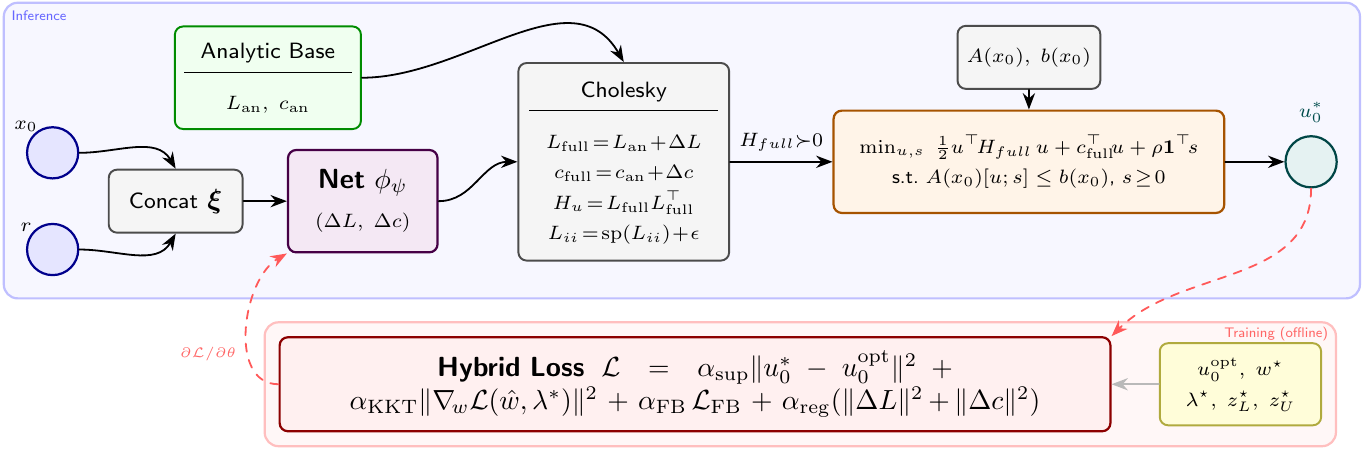
where $H \succ 0$ and $c$ are state- and reference-dependent cost parameters, hard constraints encode input bounds and affine-in-input constraints (e.g., torque limits via inverse dynamics), and the soft-constraint slack $s \geq 0$ ensures feasibility for state bounds.

This QP has only $n_z = n_u + 2n_x$ decision variables—far fewer than the full NLP—and is always feasible by construction.

---

Learning the QP Parameters: Residual-Corrector Architecture

The QP parameters $(H, c)$ must encode the entire $N$-step value function, not just the one-step stage cost. The analytic baseline $(H_\text{an}, c_\text{an})$, obtained by linearizing the output map around $x_0$, captures only the first-step contribution:

$$H_\text{an} = 2\bigl(J_\varphi^{u\top} Q\, J_\varphi^u + R\bigr), \qquad c_\text{an} = 2 J_\varphi^{u\top} Q\,(\varphi_\text{drift} - y_\text{ref}) - 2R\, u_\text{ref}.$$

A neural network $\phi_\psi$ learns the residual corrections $(\Delta L, \Delta c)$ over this baseline. The Cholesky factor $L_\text{full} = L_\text{an} + \Delta L$ yields the corrected Hessian $H(x_0) = L_\text{full} L_\text{full}^\top$, with the diagonal of $L_\text{full}$ passed through a softplus to guarantee $H(x_0) \succ 0$ for any network output. The resulting QP is solved by a differentiable interior-point layer, which provides exact constraint satisfaction and differentiable gradients through the solution.

The analytic baseline provides a warm, structured initialization; the network learns only the correction needed to match the full NLP over the remaining $N-1$ horizon steps.

---

Training: A Hybrid KKT Loss

The network is trained offline on a dataset $\mathcal{D}$ of $M$ NLP solutions with their primal-dual variables. The loss combines four terms:

Supervised imitation directly penalizes the deviation from the optimal first control action:

$$\mathcal{L}_\text{sup} = \frac{1}{M}\sum_{i=1}^M \|\hat{u}_0^{(i)} - u_0^{\star(i)}\|^2.$$

KKT stationarity penalizes violations of the first-order optimality conditions of the full NLP at the network’s prediction, using the optimal dual variables from the dataset as fixed anchors:

$$\mathcal{L}_\text{KKT} = \frac{1}{M}\sum_{i=1}^M \|\nabla_{w} \mathcal{L}(\hat{w}^{(i)},\, \mu^{\star(i)},\, \lambda^{\star(i)},\, z_L^{\star(i)},\, z_U^{\star(i)})\|^2.$$

Fischer–Burmeister complementarity enforces the complementarity and inequality feasibility conditions in smooth differentiable form via $\phi_\text{FB}(a,b) = \sqrt{a^2 + b^2} - (a+b)$, which satisfies $\phi_\text{FB}(a,b) = 0 \iff a \geq 0, b \geq 0, ab = 0$.

Regularization towards the analytic baseline prevents the learned corrections from drifting unnecessarily far.

The KKT and FB terms are evaluated at a mixed primal $\hat{w}^{(i)}$: the full optimal solution $w^{\star(i)}$ with the first control block and the resulting one-step-ahead state replaced by the network’s prediction. This gives an optimization-informed gradient signal near constraint boundaries once the supervised term has converged, at the cost of a first-order approximation in $\hat{u}_0 - u_0^\star$.

---

Case Study: Three-Link Planar Robotic Arm

We validate on a three-link planar arm with gravity ($n_x = 6$, $n_u = 3$, joint accelerations as inputs). The prediction model is a simplified double integrator $\ddot{q} = u$, while the plant is simulated with full Euler–Lagrange dynamics—representing a deliberate model mismatch. The MPC horizon is $N = 15$ steps.

The stage cost is nonlinear through the forward kinematics:

$$\ell(x, u;\, p_\text{ref}) = \|p(q) - p_\text{ref}\|_{W_{ee}}^2 + \|\dot{q}\|_{W_{dq}}^2 + \|u\|_{W_u}^2.$$

Hard constraints include torque limits enforced via inverse dynamics and acceleration bounds; state (joint position and velocity) bounds are softened. The single-step QP has $n_z = 15$ decision variables and 36 inequality rows.

The network is a three-hidden-layer MLP ($[128, 128, 64]$, ReLU), mapping an 8-dimensional input $(q, \dot{q}, p_\text{ref})$ to the 9-dimensional residual $(\Delta L, \Delta c)$. It is initialized to zero so that at startup the QP recovers the analytic one-step solution.

Training uses 100,000 samples from closed-loop IPOPT trajectories, 200 epochs with Adam and cosine learning-rate decay.

---

Results

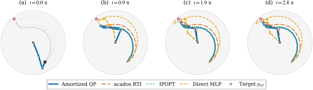
We compare against: full-horizon IPOPT (optimality reference), acados SQP-RTI (one Gauss–Newton iteration per step), and a direct MLP with identical architecture but without the differentiable QP layer.

End-effector trajectories from a common initial configuration (filled circle) to the target (star). The amortized QP closely tracks the IPOPT trajectory, while RTI and the direct MLP deviate visibly.

Metric	Amort. QP	RTI	IPOPT	Direct MLP
Mean solve time (ms)	0.116	2.453	211.8	0.095
Speedup vs. IPOPT	1826×	86×	—	2229×
Convergence	100/100	88/100	100/100	73/100
Mean EE error (m)	1.5×10⁻³	4.2×10⁻²	1.2×10⁻³	4.0×10⁻²
Mean $J_\text{cl}$ ratio vs. IPOPT	1.047	1.175	1.000	1.120
Max torque violation (N·m)	0	~0	~0	46.3
Max accel. violation (rad/s²)	0	~0	~0	20.8

The amortized policy runs in 0.116 ms on a mobile CPU—a 21× speedup over RTI and an 1826× speedup over IPOPT—while achieving closed-loop cost within 4.7% of the IPOPT optimum and converging on all 100 test scenarios. Hard constraints on torque and acceleration are satisfied to numerical precision; slack variables are active in only 0.7% of steps.

By contrast, acados RTI diverges on 12/100 scenarios, and the direct MLP converges on only 73/100 with hard constraint violations up to 46.3 N·m in torque—confirming that the differentiable QP layer is essential for both feasibility and reliability.

---

Conclusion

We have shown that, for input-affine nonlinear systems, the optimal MPC control move can be approximated by a small state-dependent QP whose parameters are predicted by a neural network. The residual-corrector architecture—analytic baseline plus learned correction, solved by a differentiable interior-point layer—achieves near-optimal closed-loop performance with guaranteed constraint satisfaction at inference times in the sub-millisecond range.

---

Footnotes

1. F. Pillitteri and A. Bemporad, “Amortized Nonlinear Model Predictive Control,” arXiv preprint arXiv:2606.05840 [eess.SY], 2026. https://arxiv.org/abs/2606.05840 ↩