A Friendly Introduction to Interior Point Methods for Constrained Optimization
 Interior
Optimization problems with constraints appear everywhere — from engineering design to machine learning and economics. Many real-world problems impose conditions like “stay within this region” or “respect a physical law,” which makes constrained optimization essential.
This page gives a concise, practical introduction to Interior Point Methods (IPMs), explains their mechanics, and shows results on a simple quadratic example.
How Interior Point Methods Work
IPMs maintain iterates strictly inside the feasible region and approach constraint boundaries only as the algorithm progresses. For inequality constraints (h(x) ≤ 0) IPMs introduce slack variables s > 0:
\[ h(x) + s = 0,\quad s > 0 \]To keep slacks positive, a logarithmic barrier is added to the objective:
\[ \phi_\tau(x,s) = f(x) - \tau \sum_i \log(s_i), \]where τ > 0 is the barrier parameter that is gradually reduced. The barrier makes the feasible interior “repulsive” near the boundary and yields a smooth optimization landscape.
Solving the Barrier Problem
Each outer iteration reduces τ and an inner solver (often a primal-dual Newton method) solves the KKT system for the barrier-augmented objective. The method updates:
- Primal variables x (decision variables)
- Dual variables (Lagrange multipliers)
Common Hessian strategies and trade-offs:
| Hessian Strategy | Pros | Cons |
|---|---|---|
| Exact Hessian | Fast convergence | Needs analytic or auto-diff |
| Gauss–Newton | Efficient for least-squares | Problem-specific |
| BFGS (quasi-Newton) | Lower memory | Accumulates approximation error |
| Steepest Descent | Simple and robust | Slow convergence |
Why use Interior Point Methods?
- Smooth, stable iterates that avoid frequent constraint switching
- Scales well for many large linear and convex problems
- Used in solvers like IPOPT, MOSEK, and KNITRO
Caveats: requires tuning of the barrier schedule and relies on good linear algebra (factorizations, preconditioning).
Example: Quadratic Optimization with Equality and Inequality Constraints
Problem:
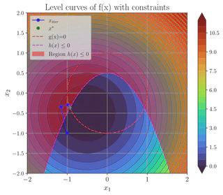
\[ \begin{aligned} \min_x &\quad f(x) = x^\top x + \mathbf{1}^\top x \\ \text{s.t.} &\quad g(x) = x^\top x - 1 = 0 \\ &\quad h(x) = 0.5 - x_1^2 - x_2 \le 0 \end{aligned} \]The solver was run from different initial guesses to illustrate typical behavior.
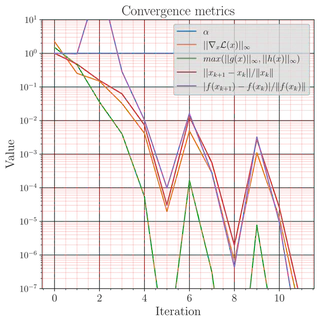
Initial guess x₀ = [-1, -1]^T
Optimization path (level sets and iterates):
Convergence metrics (objective, residuals, τ schedule):
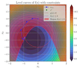
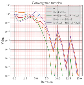
Initial guess x₀ = [0, 1]^T
Optimization path:
Convergence metrics:
Additional initial conditions tested
- x₀ = [0.5, 0.0]^T — feasible interior start
- x₀ = [2.0, 2.0]^T — far exterior start (projected inward by barrier)
- Random seeds to assess robustness across basins of attraction
The experiments show consistent interior progress, with convergence speed depending on starting proximity to the constraint boundary and the chosen Hessian approximation.
Takeaways
- IPMs produce smooth, predictable progress by staying in the feasible interior and relying on barrier terms.
- Barrier parameter scheduling and linear algebra quality are key to performance.
- For many practical problems, off-the-shelf IPM solvers provide a reliable solution path.
For reproducibility: include the solver settings (τ schedule, termination tolerances, Hessian choice) and initial seeds when sharing results.